3. Feature Engineering (with Visuals)

This notebook adds and visualizes new features.

import pandas as pd
import matplotlib.pyplot as plt
import seaborn as sns
from sklearn.preprocessing import StandardScaler

# Load cleaned data
df = pd.read_csv("processed_cleveland_clean.csv")

##Initial Distributions of Key Features

num_cols = ['age', 'trestbps', 'chol', 'thalach', 'oldpeak']
df[num_cols].hist(bins=20, figsize=(14, 8))
plt.suptitle("Initial Numerical Feature Distributions", y=1.02)
plt.tight_layout()
plt.show()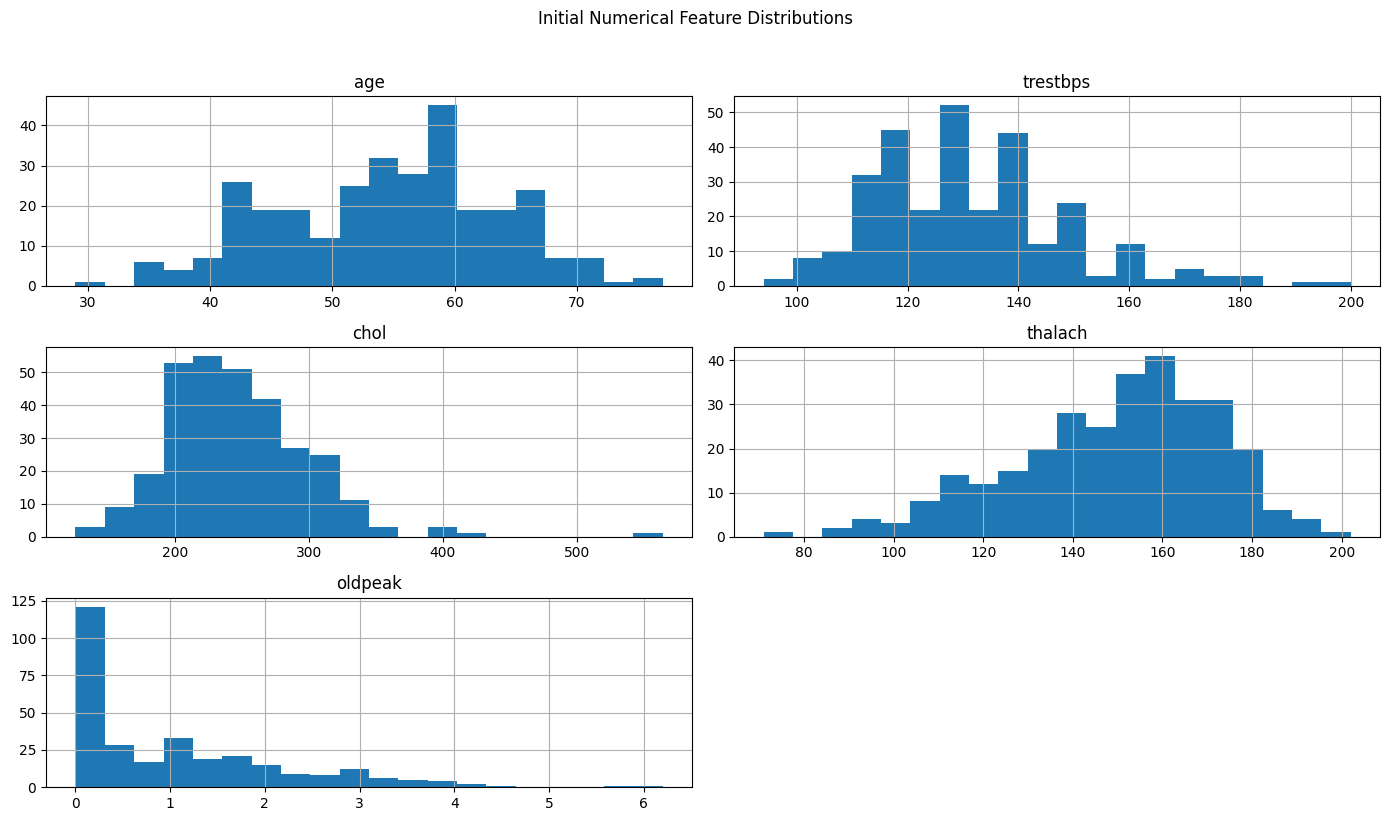

##Add Engineered Features

df["chol_per_age"] = df["chol"] / df["age"]
df["stress_index"] = df["thalach"] / (df["oldpeak"] + 1)
df["bp_dev"] = df["trestbps"] - 120
df["age_bucket"] = pd.cut(df["age"], bins=[29, 40, 55, 70, 100], labels=[0, 1, 2, 3])
df = pd.get_dummies(df, columns=["age_bucket"], drop_first=True)
df.head()

	age	sex	cp	trestbps	chol	fbs	restecg	thalach	exang	oldpeak	slope	ca	thal	num	chol_per_age	stress_index	bp_dev	age_bucket_1	age_bucket_2	age_bucket_3
0	63.0	1.0	1.0	145.0	233.0	1.0	2.0	150.0	0.0	2.3	3.0	0.0	6.0	0	3.698413	45.454545	25.0	False	True	False
1	67.0	1.0	4.0	160.0	286.0	0.0	2.0	108.0	1.0	1.5	2.0	3.0	3.0	2	4.268657	43.200000	40.0	False	True	False
2	67.0	1.0	4.0	120.0	229.0	0.0	2.0	129.0	1.0	2.6	2.0	2.0	7.0	1	3.417910	35.833333	0.0	False	True	False
3	37.0	1.0	3.0	130.0	250.0	0.0	0.0	187.0	0.0	3.5	3.0	0.0	3.0	0	6.756757	41.555556	10.0	False	False	False
4	41.0	0.0	2.0	130.0	204.0	0.0	2.0	172.0	0.0	1.4	1.0	0.0	3.0	0	4.975610	71.666667	10.0	True	False	False

##Distributions of Engineered Features

import matplotlib.pyplot as plt

eng_cols = {
    "chol_per_age": "Cholesterol Per Age",
    "stress_index": "Stress Index",
    "bp_dev": "BP Deviation"
}

# Create custom subplots with proper titles
fig, axes = plt.subplots(1, 3, figsize=(18, 5))

for ax, (col, label) in zip(axes, eng_cols.items()):
    ax.hist(df[col], bins=20, color="skyblue", edgecolor="black")
    ax.set_title(label)
    ax.set_xlabel(label)
    ax.set_ylabel("Frequency")

plt.suptitle("Engineered Feature Distributions", fontsize=16, y=1.05)
plt.tight_layout()
plt.show()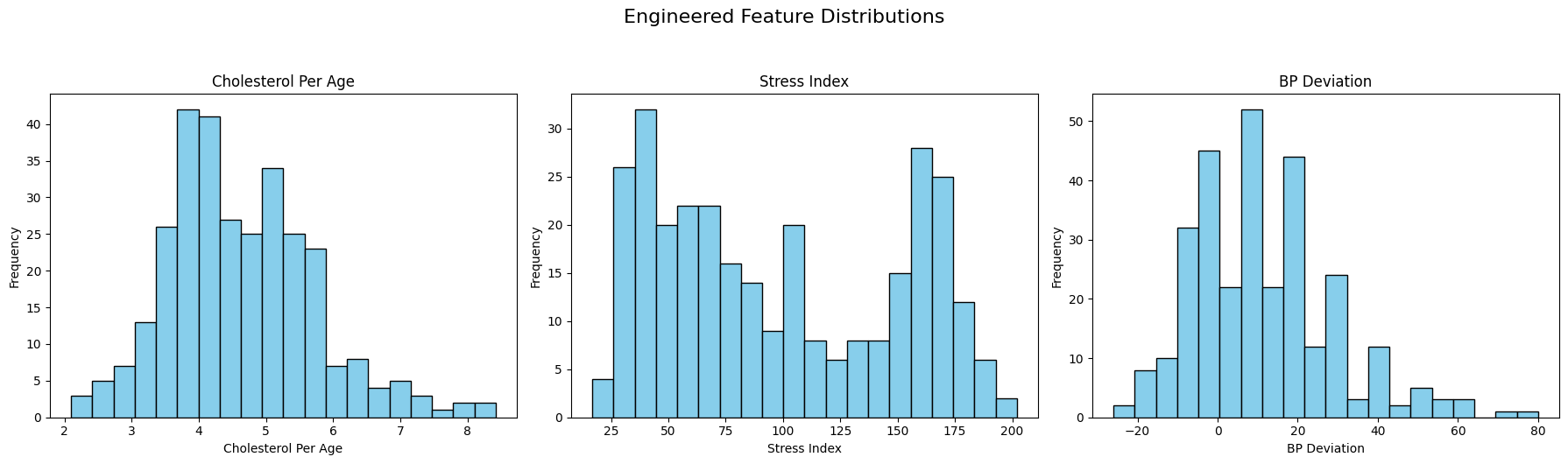

##Boxplots by Target

fig, axes = plt.subplots(1, 3, figsize=(18, 5))
for i, col in enumerate(eng_cols):
    sns.boxplot(data=df, x='num', y=col, ax=axes[i])
    axes[i].set_title(f"{col} by Target")
plt.tight_layout()
plt.show()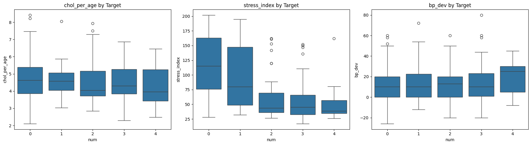

##Scale Numerical Features

scale_cols = ['age', 'trestbps', 'chol', 'thalach', 'oldpeak',
              'chol_per_age', 'stress_index', 'bp_dev']
scaler = StandardScaler()
df[scale_cols] = scaler.fit_transform(df[scale_cols])
df.head()

	age	sex	cp	trestbps	chol	fbs	restecg	thalach	exang	oldpeak	slope	ca	thal	num	chol_per_age	stress_index	bp_dev	age_bucket_1	age_bucket_2	age_bucket_3
0	0.948726	1.0	1.0	0.757525	-0.264900	1.0	2.0	0.017197	0.0	1.087338	3.0	0.0	6.0	0	-0.846084	-1.016799	0.757525	False	True	False
1	1.392002	1.0	4.0	1.611220	0.760415	0.0	2.0	-1.821905	1.0	0.397182	2.0	3.0	3.0	2	-0.329103	-1.059948	1.611220	False	True	False
2	1.392002	1.0	4.0	-0.665300	-0.342283	0.0	2.0	-0.902354	1.0	1.346147	2.0	2.0	7.0	1	-1.100386	-1.200934	-0.665300	False	True	False
3	-1.932564	1.0	3.0	-0.096170	0.063974	0.0	0.0	1.637359	0.0	2.122573	3.0	0.0	3.0	0	1.926599	-1.091420	-0.096170	False	False	False
4	-1.489288	0.0	2.0	-0.096170	-0.825922	0.0	2.0	0.980537	0.0	0.310912	1.0	0.0	3.0	0	0.311818	-0.515143	-0.096170	True	False	False

##Save Feature-Engineered Dataset

df.to_csv("engineered_heart_data.csv", index=False)
print("✅ Feature engineered data saved as 'engineered_heart_data.csv'")